Add Lowess Curve
This operation is only available in the right-click menus of scatterplots and sum-difference plots. What it does depends on if there is a ✓ mark to its left in a right-click menu.
- When there is no ✓ mark:
It adds a lowess curve to the point cloud to help you better perceive the relationship between the 2 variables plotted on the horizontal and the vertical axes.
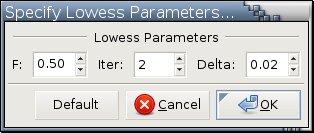
If the Shift key is held down when this operation is invoked from the right-click menu [1], a dialog like
will pop up for you to specify the following 3 parameters: F specifies the amount of smoothing and is
the fraction of points used to compute each
fitted value.
As F increases the curve becomes smoother.
Choosing F in the range 0.2 to 0.8 usually results in
a good fit.
The default is 0.5.
F specifies the amount of smoothing and is
the fraction of points used to compute each
fitted value.
As F increases the curve becomes smoother.
Choosing F in the range 0.2 to 0.8 usually results in
a good fit.
The default is 0.5.
 Iter is the number of iterations in the robust fit.
If Iter is 0, the nonrobust fit is returned.
Setting Iter equal to 2, the default, should serve most purposes.
Iter is the number of iterations in the robust fit.
If Iter is 0, the nonrobust fit is returned.
Setting Iter equal to 2, the default, should serve most purposes.
 Delta is a number between 0.0 and 1.0 and
may be used to save computations.
If the number of points of unique X coordinates
is less than 100, set Delta equal to 0.0.
If there are more than 100 points of unique X coordinates,
setting Delta to 0.02, the default, often works well.
Read this footnote
[2]
for more information on how to choose Delta.
Delta is a number between 0.0 and 1.0 and
may be used to save computations.
If the number of points of unique X coordinates
is less than 100, set Delta equal to 0.0.
If there are more than 100 points of unique X coordinates,
setting Delta to 0.02, the default, often works well.
Read this footnote
[2]
for more information on how to choose Delta.
If the Shift key is not held down when this operation is invoked, a lowess curve will be fitted and drawn using either the lowess parameters specified last time when Shift-<Add Lowess Curve> is invoked or the default values (0.5 for F, 2 for Iter, and 0.02 for Delta) if Shift-<Add Lowess Curve> has never been invoked.
- When there is a ✓ mark:
The plot on which this operation is invoked is already displaying a lowess curve. This operation will remove the lowess curve being displayed.
If this operation is invoked from a panel plot [3] of a trellis display, the end effect is equivalent to invoking Add Lowess Curves on the associated trellis display.